软硬约束下的轨迹生成：理论与代码分析

本项目代码：

github.com/liangwq/robot_motion_planing

轨迹约束中的软硬约束

前面的几篇文章已经介绍了，轨迹约束的本质就是在做带约束的轨迹拟合。输入就是waypoint点list，约束条件有两种硬约束和软约束。所谓硬约束对应到数学形式就是代价函数，硬约束对应的就是最优化秋季的约束条件部分。对应到物理意义就是，为了获得机器人可行走的安全的轨迹有：

1. 把轨迹通过代价函数推离障碍物的方式
2. 给出障碍物之间的可行走凸包走廊，通过硬约束让机器人轨迹必须在凸包走廊行走

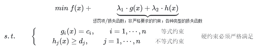
上图展示的是软硬约束下Bezier曲线拟合的求解的数学框架，以及如何把各种的约束条件转成数学求解的代价函数（软约束）或者是求解的约束条件（软约束）。image.png

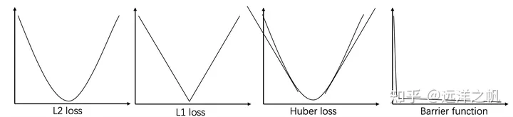
上面是对常用的代价函数约束的几种表示方式的举例。image.png

Bezier曲线拟合轨迹

前面已经一篇文章介绍过贝赛尔曲线拟合的各种优点：

• 端点插值。贝塞尔曲线始终从第一个控制点开始，结束于最后一个控制点，并且不会经过任何其他控制点。
• 凸包。贝塞尔曲线 ( ) 由一组控制点 完全限制在由所有这些控制点定义的凸包内。
• 速度曲线。贝塞尔曲线 ( ) 的导数曲线 ′( ) 被称为速度曲线，它也是一个由控制点定义的贝塞尔曲线，其中控制点为 ∙ ( +1− )，其中 是阶数。
• 固定时间间隔。贝塞尔曲线始终在 [0,1] 上定义。

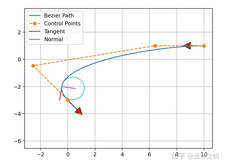
Fig1.一段轨迹用bezier曲线拟合image.png

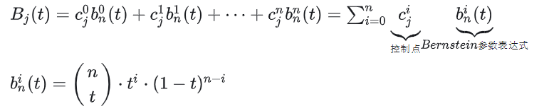
上面的两个表达式对应的代码实现如下：

def bernstein_poly(n, i, t):"""Bernstein polynom.:param n: (int) polynom degree:param i: (int):param t: (float):return: (float)"""return scipy.special.comb(n, i) * t ** i * (1 - t) ** (n - i)def bezier(t, control_points):"""Return one point on the bezier curve.:param t: (float) number in [0, 1]:param control_points: (numpy array):return: (numpy array) Coordinates of the point"""n = len(control_points) - 1return np.sum([bernstein_poly(n, i, t) * control_points[i] for i in range(n + 1)], axis=0)

要用Bezier曲线来表示一段曲线，上面已经给出了表达式和代码实现，现在缺的就是给定控制点，把控制点带进来用Bezier曲线表达式来算出给定终点和结束点中需要画的点坐标。下面代码给出了4个控制点、6个控制点的Bezier曲线实现；其中为了画曲线需要算170个线上点。代码如下：

def calc_4points_bezier_path(sx, sy, syaw, ex, ey, eyaw, offset):"""Compute control points and path given start and end position.:param sx: (float) x-coordinate of the starting point:param sy: (float) y-coordinate of the starting point:param syaw: (float) yaw angle at start:param ex: (float) x-coordinate of the ending point:param ey: (float) y-coordinate of the ending point:param eyaw: (float) yaw angle at the end:param offset: (float):return: (numpy array, numpy array)"""dist = np.hypot(sx - ex, sy - ey) / offsetcontrol_points = np.array([[sx, sy], [sx + dist * np.cos(syaw), sy + dist * np.sin(syaw)], [ex - dist * np.cos(eyaw), ey - dist * np.sin(eyaw)], [ex, ey]])path = calc_bezier_path(control_points, n_points=170)return path, control_pointsdef calc_6points_bezier_path(sx, sy, syaw, ex, ey, eyaw, offset):"""Compute control points and path given start and end position.:param sx: (float) x-coordinate of the starting point:param sy: (float) y-coordinate of the starting point:param syaw: (float) yaw angle at start:param ex: (float) x-coordinate of the ending point:param ey: (float) y-coordinate of the ending point:param eyaw: (float) yaw angle at the end:param offset: (float):return: (numpy array, numpy array)"""dist = np.hypot(sx - ex, sy - ey) * offsetcontrol_points = np.array([[sx, sy], [sx + 0.25 * dist * np.cos(syaw), sy + 0.25 * dist * np.sin(syaw)], [sx + 0.40 * dist * np.cos(syaw), sy + 0.40 * dist * np.sin(syaw)], [ex - 0.40 * dist * np.cos(eyaw), ey - 0.40 * dist * np.sin(eyaw)], [ex - 0.25 * dist * np.cos(eyaw), ey - 0.25 * dist * np.sin(eyaw)], [ex, ey]])path = calc_bezier_path(control_points, n_points=170)return path, control_pointsdef calc_bezier_path(control_points, n_points=100):"""Compute bezier path (trajectory) given control points.:param control_points: (numpy array):param n_points: (int) number of points in the trajectory:return: (numpy array)"""traj = []for t in np.linspace(0, 1, n_points):traj.append(bezier(t, control_points))return np.array(traj)

有了一段Bezier曲线的拟合方式，接下来要做的就是如何生成多段Bezier曲线合成一条轨迹；并且是需要可以通过代价函数方式（软约束）+必须经过指定点+制定点衔接要连续（硬约束）来生成一条光滑的轨迹曲线。

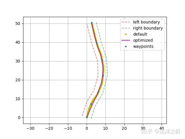
Fig2.无障碍物，带bondary轨迹做了smooth优化Figure_1.png

多段Bezier曲线生成代码如下，其实原理很简单，给定多个waypoint点，每相邻两个wayponit生成一段Bezizer曲线，代码如下：

# Bezier path one as per the approach suggested in# https://users.soe.ucsc.edu/~elkaim/Documents/camera_WCECS2008_IEEE_ICIAR_58.pdfdef cubic_bezier_path(self, ax, ay):dyaw, _ = self.calc_yaw_curvature(ax, ay)cx = []cy = []ayaw = dyaw.copy()for n in range(1, len(ax)-1):yaw = 0.5*(dyaw[n] + dyaw[n-1])ayaw[n] = yawlast_ax = ax[0]last_ay = ay[0]last_ayaw = ayaw[0]# for n waypoints, there are n-1 bezier curvesfor i in range(len(ax)-1):path, ctr_points = calc_4points_bezier_path(last_ax, last_ay, ayaw[i], ax[i+1], ay[i+1], ayaw[i+1], 2.0)cx = np.concatenate((cx, path.T[0][:-2]))cy = np.concatenate((cy, path.T[1][:-2]))cyaw, k = self.calc_yaw_curvature(cx, cy)last_ax = path.T[0][-1]last_ay = path.T[1][-1]return cx, cy

代价函数计算包括：曲率代价 + 偏差代价 + 距离代价 + 连续性代价，同时还有边界条件，轨迹必须在tube内的不等式约束，以及问题优化求解。具体代码实现如下：

# Objective function of cost to be minimizeddef cubic_objective_func(self, deviation):ax = self.waypoints.x.copy()ay = self.waypoints.y.copy()for n in range(0, len(deviation)):ax[n+1] -= deviation[n]*np.sin(self.waypoints.yaw[n+1])ay[n+1] += deviation[n]*np.cos(self.waypoints.yaw[n+1])bx, by = self.cubic_bezier_path(ax, ay)yaw, k = self.calc_yaw_curvature(bx, by)# cost of curvature continuityt = np.zeros((len(k)))dk = self.calc_d(t, k)absolute_dk = np.absolute(dk)continuity_cost = 10.0 * np.mean(absolute_dk)# curvature costabsolute_k = np.absolute(k)curvature_cost = 14.0 * np.mean(absolute_k)# cost of deviation from input waypointsabsolute_dev = np.absolute(deviation)deviation_cost = 1.0 * np.mean(absolute_dev)distance_cost = 0.5 * self.calc_path_dist(bx, by)return curvature_cost + deviation_cost + distance_cost + continuity_cost# Minimize objective function using scipy optimize minimizedef optimize_min_cubic(self):print("Attempting optimization minima")initial_guess = [0, 0, 0, 0, 0]bnds = ((-self.bound, self.bound), (-self.bound, self.bound), (-self.bound, self.bound), (-self.bound, self.bound), (-self.bound, self.bound))result = optimize.minimize(self.cubic_objective_func, initial_guess, bounds=bnds)ax = self.waypoints.x.copy()ay = self.waypoints.y.copy()if result.success:print("optimized true")deviation = result.xfor n in range(0, len(deviation)):ax[n+1] -= deviation[n]*np.sin(self.waypoints.yaw[n+1])ay[n+1] += deviation[n]*np.cos(self.waypoints.yaw[n+1])x, y = self.cubic_bezier_path(ax, ay)yaw, k = self.calc_yaw_curvature(x, y)self.optimized_path = Path(x, y, yaw, k)else:print("optimization failure, defaulting")exit()

带障碍物的Bezier曲线轨迹生

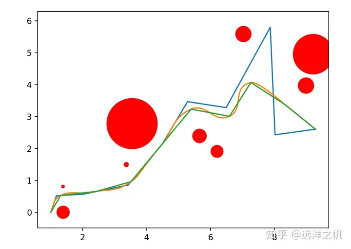
带有障碍物的场景，通过代价函数让生成的曲线远离障碍物。从而得到一条可以安全行走的轨迹，下面是具体的代码实现。optimizer_k中lambda函数f就是在求解轨迹在经过障碍物附近时候的代价，penalty1、penalty2就是在求曲线经过障碍物附近的具体代价值；
b.arc_len(granuality=10)+B.arc_len(granuality=10)+m_k + penalty1 + penalty2就是轨迹的整体代价。for循环部分用scipy的optimize的minimize来求解轨迹。

def optimizer_k(cd, k, path, i, obs, curve_penalty_multiplier, curve_penalty_divider, curve_penalty_obst):"""Bezier curve optimizer that optimizes the curvature and path length by changing the distance of p1 and p2 from points p0 and p3, respectively. """p_tmp = copy.deepcopy(path)if i+3 > len(path)-1:b = CubicBezier()b.p0 = p_tmp[i]x, y = calc_p1(p_tmp[i], p_tmp[i + 1], p_tmp[i - 1], i, cd[0])b.p1 = Point(x, y)x, y = calc_p2(p_tmp[i-1], p_tmp[i + 0], p_tmp[i + 1], i, cd[1])b.p2 = Point(x, y)b.p3 = p_tmp[i + 1]B = CubicBezier()else:b = CubicBezier()b.p0 = p_tmp[i]x, y = calc_p1(p_tmp[i],p_tmp[i+1],p_tmp[i-1], i, cd[0])b.p1 = Point(x, y)x, y = calc_p2(p_tmp[i],p_tmp[i+1],p_tmp[i+2], i, cd[1])b.p2 = Point(x, y)b.p3 = p_tmp[i + 1]B = CubicBezier()B.p0 = p_tmp[i]x, y = calc_p1(p_tmp[i+1], p_tmp[i + 2], p_tmp[i], i, 10)B.p1 = Point(x, y)x, y = calc_p2(p_tmp[i+1], p_tmp[i + 2], p_tmp[i + 3], i, 10)B.p2 = Point(x, y)B.p3 = p_tmp[i + 1]m_k = b.max_k()if m_k>k:m_k= m_k*curve_penalty_multiplierelse:m_k = m_k/curve_penalty_dividerf = lambda x, y: max(math.sqrt((x[0] - y[0].x) ** 2 + (x[1] - y[0].y) ** 2) * curve_penalty_obst, 10) if math.sqrt((x[0] - y[0].x) ** 2 + (x[1] - y[0].y) ** 2) < y[1] else 0b_t = b.calc_curve(granuality=10)b_t = zip(b_t[0],b_t[1])B_t = B.calc_curve(granuality=10)B_t = zip(B_t[0], B_t[1])penalty1 = 0penalty2 = 0for o in obs:for t in b_t:penalty1 = max(penalty1,f(t,o))for t in B_t:penalty2 = max(penalty2,f(t,o))return b.arc_len(granuality=10)+B.arc_len(granuality=10)+m_k + penalty1 + penalty2# Optimize the initial path for n_path_opt cyclesfor m in range(n_path_opt):if m%2:for i in range(1,len(path)-1):x0 = [0.0, 0.0]bounds = Bounds([-1, -1], [1, 1])res = minimize(optimizer_p, x0, args=(path, i, obs, path_penalty), method='TNC', tol=1e-7, bounds=bounds)x, y = res.xpath[i].x += xpath[i].y += yelse:for i in range(len(path)-1,1):x0 = [0.0, 0.0]bounds = Bounds([-1, -1], [1, 1])res = minimize(optimizer_p, x0, args=(path, i, obs, path_penalty), method='TNC', tol=1e-7, bounds=bounds)x, y = res.xpath[i].x += xpath[i].y += y

带飞行走廊的Bezier轨迹生成

得益于贝赛尔曲线拟合的优势，如果我们可以让机器人可行走的轨迹转成多个有重叠区域的凸多面体，那么轨迹完全位于飞行走廊内。

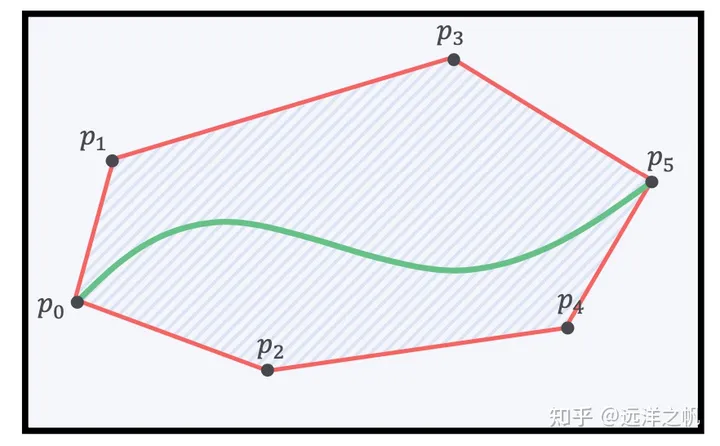
image.png

• 飞行走廊由凸多边形组成。
• 每个立方体对应于一段贝塞尔曲线。
• 此曲线的控制点被强制限制在多边形内部。
• 轨迹完全位于所有点的凸包内。

如何通过把障碍物地图生成可行凸包走廊

生成凸包走廊的方法目前有以下三大类的方法：

平行凸簇膨胀方法

从栅格地图出发，利用最小凸集生成算法，完成凸多面体的生成。其算法的思想是首先获得一个凸集，再沿着凸集的表面进行扩张，扩张之后再进行凸集检测，判断新扩张的集合是否保持为凸。一直扩张到不能再扩张为止，再提取凸集的边缘点，利用快速凸集生成算法，生成凸多面体。该算法的好处在于可以利用这种扩张的思路，将安全的多面体的体积尽可能的充满整个空间，因此获得的安全通道更大。但其也具有一定的缺点，就是计算量比较大，计算所需要的时间比较长，为了解决这个问题，在该文章中，又提出了采用GPU加速的方法，来加速计算。

基于凸分解的安全通道生成

基于凸分解的安全通道生成方法由四个步骤完成安全通道的生成，分别为：找到椭球、找到多面体、边界框、收缩。

半定规划的迭代区域膨胀

为了获取多面体，这个方法首先构造一个初始椭球，由一个以选定点为中心的单位球组成。然后，遍历障碍物，为每个障碍物生成一个超平面，该超平面与障碍物相切并将其与椭球分开。再次，这些超平面定义了一组线性约束，它们的交集是一个多面体。然后，可以在那个多面体中找到一个最大的椭球，使用这个椭球来定义一组新的分离超平面，从而定义一个新的多面体。选择生成分离超平面的方法，这样椭圆体的体积在迭代之间永远不会减少。可以重复这个过程，直到椭圆体的增长率低于某个阈值，此时我们返回多面体和内接椭圆体。这个方法具有迭代的思想，并且具有收敛判断的标准，算法的收敛快慢和初始椭球具有很大的关系。

Fig3.半定规划的迭代区域膨胀。每一行即为一次迭代操作，直到椭圆体的增长率低于阈值。image.png

这篇文章介绍的是“半定规划的迭代区域膨胀”方法，具体代码实现如下：

# 根据输入路径对空间进行凸分解def decomp(self, line_points: list[np.array], obs_points: list[np.array], visualize=True):# 最终结果decomp_polygons = list()# 构建输入障碍物点的kdtreeobs_kdtree = KDTree(obs_points)# 进行空间分解for i in range(len(line_points) - 1):# 得到当前线段pf, pr = line_points[i], line_points[i + 1]print(pf)print(pr)# 构建初始多面体init_polygon = self.initPolygon(pf, pr)print(init_polygon.getInterPoints())print(init_polygon.getVerticals())# 过滤障碍物点candidate_obs_point_indexes = obs_kdtree.query_ball_point((pf + pr) / 2, np.linalg.norm([np.linalg.norm(pr - pf) / 2 + self.consider_range_, self.consider_range_]))local_obs_points = list()for index in candidate_obs_point_indexes:if init_polygon.inside(obs_points[index]):local_obs_points.append(obs_points[index])# 得到初始椭圆ellipse = self.findEllipse(pf, pr, local_obs_points)# 根据初始椭圆构建多面体polygon = self.findPolygon(ellipse, init_polygon, local_obs_points)# 进行保存decomp_polygons.append(polygon)if visualize:# 进行可视化plt.figure()# 绘制路径段plt.plot([pf[1], pr[1]], [pf[0], pr[0]], color="red")# 绘制初始多面体verticals = init_polygon.getVerticals()# 绘制多面体顶点plt.plot([v[1] for v in verticals] + [verticals[0][1]], [v[0] for v in verticals] + [verticals[0][0]], color="blue", linestyle="--")# 绘制障碍物点plt.scatter([p[1] for p in local_obs_points], [p[0] for p in local_obs_points], marker="o")# 绘制椭圆ellipse_x, ellipse_y = list(), list()for theta in np.linspace(-np.pi, np.pi, 1000):raw_point = np.array([np.cos(theta), np.sin(theta)])ellipse_point = np.dot(ellipse.C_, raw_point) + ellipse.d_ellipse_x.append(ellipse_point[0])ellipse_y.append(ellipse_point[1])plt.plot(ellipse_y, ellipse_x, color="orange")# 绘制最终多面体# 得到多面体顶点verticals = polygon.getVerticals()# 绘制多面体顶点plt.plot([v[1] for v in verticals] + [verticals[0][1]], [v[0] for v in verticals] + [verticals[0][0]], color="green")plt.show()return decomp_polygons# 构建初始多面体def initPolygon(self, pf: np.array, pr: np.array) -> Polygon:# 记录多面体的平面polygon_planes = list()# 得到线段方向向量dire = self.normalize(pr - pf)# 得到线段法向量dire_h = np.array([dire[1], -dire[0]])# 得到平行范围p_1 = pf + self.consider_range_ * dire_hp_2 = pf - self.consider_range_ * dire_hpolygon_planes.append(Hyperplane(dire_h, p_1))polygon_planes.append(Hyperplane(-dire_h, p_2))# 得到垂直范围p_3 = pr + self.consider_range_ * direp_4 = pf - self.consider_range_ * direpolygon_planes.append(Hyperplane(dire, p_3))polygon_planes.append(Hyperplane(-dire, p_4))# 构建多面体polygon = Polygon(polygon_planes)return polygon# 得到初始椭圆def findEllipse(self, pf: np.array, pr: np.array, obs_points: list[np.array]) -> Ellipse:# 计算长轴long_axis_value = np.linalg.norm(pr - pf) / 2axes = np.array([long_axis_value, long_axis_value])# 计算旋转rotation = self.vec2Rotation(pr - pf)# 计算初始椭圆C = np.dot(rotation, np.dot(np.array([[axes[0], 0], [0, axes[1]]]), np.transpose(rotation)))d = (pr + pf) / 2ellipse = Ellipse(C, d)# 得到椭圆内的障碍物点inside_obs_points = ellipse.insidePoints(obs_points)# 对椭圆进行调整，使得全部障碍物点都在椭圆外while inside_obs_points:# 得到与椭圆距离最近的点closest_obs_point = ellipse.closestPoint(inside_obs_points)# 将最近点转到椭圆坐标系下closest_obs_point = np.dot(np.transpose(rotation), closest_obs_point - ellipse.d_) # 根据最近点，在椭圆长轴不变的情况下对短轴进行改变，使得，障碍物点在椭圆上if Compare.small(closest_obs_point[0], axes[0]):axes[1] = np.abs(closest_obs_point[1]) / np.sqrt(1 - (closest_obs_point[0] / axes[0]) ** 2)# 更新椭圆ellipse.C_ = np.dot(rotation, np.dot(np.array([[axes[0], 0], [0, axes[1]]]), np.transpose(rotation)))# 更新椭圆内部障碍物inside_obs_points = ellipse.insidePoints(inside_obs_points, include_bound=False)return ellipse# 进行多面体的构建def findPolygon(self, ellipse: Ellipse, init_polygon: Polygon, obs_points: list[np.array]) -> Polygon:# 多面体由多个超平面构成polygon_planes = copy.deepcopy(init_polygon.hyper_planes_)# 初始化范围超平面remain_obs_points = obs_pointswhile remain_obs_points:# 得到与椭圆最近障碍物closest_point = ellipse.closestPoint(remain_obs_points)# 计算该处的切平面的法向量norm_vector = np.dot(np.linalg.inv(ellipse.C_), np.dot(np.linalg.inv(ellipse.C_), (closest_point - ellipse.d_)))norm_vector = self.normalize(norm_vector)# 构建平面hyper_plane = Hyperplane(norm_vector, closest_point)# 保存到多面体平面中polygon_planes.append(hyper_plane)# 去除切平面外部的障碍物new_remain_obs_points = list()for point in remain_obs_points:if Compare.small(hyper_plane.signDist(point), 0):new_remain_obs_points.append(point)remain_obs_points = new_remain_obs_pointspolygon = Polygon(polygon_planes)return polygon

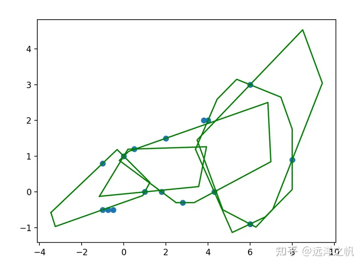
上面图是给定16个障碍物点，必经6个路径点后得到的凸包可行走廊，具体代码如下：

def main():# 路径点line_points = [np.array([-1.5, 0.0]), np.array([0.0, 0.8]), np.array([1.5, 0.3]), np.array([5, 0.6]), np.array([6, 1.2]), np.array([7.6, 2.2])]# 障碍物点obs_points = [np.array([4, 2.0]),np.array([6, 3.0]),np.array([2, 1.5]),np.array([0, 1]),np.array([1, 0]),np.array([1.8, 0]),np.array([3.8, 2]),np.array([0.5, 1.2]),np.array([4.3, 0]),np.array([8, 0.9]),np.array([2.8, -0.3]),np.array([6, -0.9]),np.array([-0.5, -0.5]),np.array([-0.75 ,-0.5]),np.array([-1, -0.5]),np.array([-1, 0.8])]convex_decomp = ConvexDecomp(2)decomp_polygons = convex_decomp.decomp(line_points, obs_points, False)#convex_decomp.decomp(line_points, obs_points,False)plt.figure()# 绘制障碍物点plt.scatter([p[0] for p in obs_points], [p[1] for p in obs_points], marker="o")# 绘制边界for polygon in decomp_polygons:verticals = polygon.getVerticals()# 绘制多面体顶点plt.plot([v[0] for v in verticals] + [verticals[0][0]], [v[1] for v in verticals] + [verticals[0][1]], color="green")#plt.plot(x_samples, y_samples)plt.show()

带凸包走廊求解

带凸包走廊的光滑轨迹生成。前面已经求解得到了可行的凸包走廊，这部分可以做为硬约束作为最优化求解的不等式条件。要求的光滑路径和必须经过点的点，这部分可以把必须经过点作为等式约束，光滑路径可以通过代价函数来实现。这样就可以把带软硬约束的轨迹生成框架各种技能点都用上了。

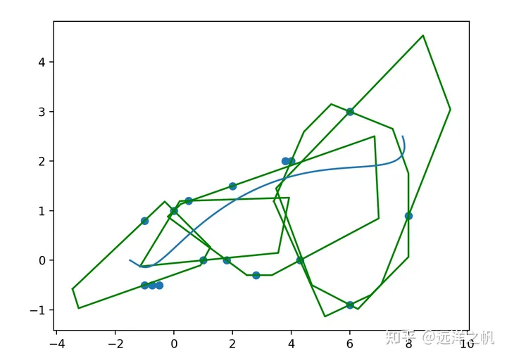
下面看具体代码实现：

# 进行优化def optimize(self, start_state: np.array, end_state: np.array, line_points: list[np.array], polygons: list[Polygon]):assert(len(line_points) == len(polygons) + 1)# 得到分段数量segment_num = len(polygons)assert(segment_num >= 1)# 计算初始时间分配time_allocations = list()for i in range(segment_num):time_allocations.append(np.linalg.norm(line_points[i+1] - line_points[i]) / self.vel_max_)# 进行优化迭代max_inter = 10cur_iter = 0while cur_iter < max_inter:# 进行轨迹优化piece_wise_trajectory = self.optimizeIter(start_state, end_state, polygons, time_allocations, segment_num)# 对优化轨迹进行时间调整，以保证轨迹满足运动上限约束cur_iter += 1# 计算每一段轨迹的最大速度，最大加速度，最大jerkcondition_fit = Truefor n in range(segment_num):# 得到最大速度，最大加速度，最大jerkt_samples = np.linspace(0, time_allocations[n], 100)v_max, a_max, j_max = self.vel_max_, self.acc_max_, self.jerk_max_for t_sample in t_samples:v_max = max(v_max, np.abs(piece_wise_trajectory.trajectory_segments_[n][0].derivative(t_sample)), np.abs(piece_wise_trajectory.trajectory_segments_[n][1].derivative(t_sample)))a_max = max(a_max, np.abs(piece_wise_trajectory.trajectory_segments_[n][0].secondOrderDerivative(t_sample)), np.abs(piece_wise_trajectory.trajectory_segments_[n][1].secondOrderDerivative(t_sample)))j_max = max(j_max, np.abs(piece_wise_trajectory.trajectory_segments_[n][0].thirdOrderDerivative(t_sample)), np.abs(piece_wise_trajectory.trajectory_segments_[n][1].thirdOrderDerivative(t_sample)))# 判断是否满足约束条件if Compare.large(v_max, self.vel_max_) or Compare.large(a_max, self.acc_max_) or Compare.large(j_max, self.jerk_max_):ratio = max(1, v_max / self.vel_max_, (a_max / self.acc_max_)**0.5, (j_max / self.jerk_max_)**(1/3))time_allocations[n] = ratio * time_allocations[n]condition_fit = Falseif condition_fit:breakreturn piece_wise_trajectory# 优化迭代def optimizeIter(self, start_state: np.array, end_state: np.array, polygons: list[Polygon], time_allocations: list, segment_num):# 构建目标函数 inter (jerk)^2inte_jerk_square = np.array([[720.0, -1800.0, 1200.0, 0.0, 0.0, -120.0],[-1800.0, 4800.0, -3600.0, 0.0, 600.0, 0.0],[1200.0, -3600.0, 3600.0, -1200.0, 0.0, 0.0],[0.0, 0.0, -1200.0, 3600.0, -3600.0, 1200.0],[0.0, 600.0, 0.0, -3600.0, 4800.0, -1800.0],[-120.0, 0.0, 0.0, 1200.0, -1800.0, 720.0]])# 二次项系数P = np.zeros((self.dim_ * segment_num * self.freedom_, self.dim_ * segment_num * self.freedom_))for sigma in range(self.dim_):for n in range(segment_num):for i in range(self.freedom_):for j in range(self.freedom_):index_i = sigma * segment_num * self.freedom_ + n * self.freedom_ + iindex_j = sigma * segment_num * self.freedom_ + n * self.freedom_ + jP[index_i][index_j] = inte_jerk_square[i][j] / (time_allocations[n] ** 5)P = P * 2P = sparse.csc_matrix(P)# 一次项系数q = np.zeros((self.dim_ * segment_num * self.freedom_,))# 构建约束条件equality_constraints_num = 5 * self.dim_ + 3 * (segment_num - 1) * self.dim_inequality_constraints_num = 0for polygon in polygons:inequality_constraints_num += self.freedom_ * len(polygon.hyper_planes_)A = np.zeros((equality_constraints_num + inequality_constraints_num, self.dim_ * segment_num * self.freedom_))lb = -float("inf") * np.ones((equality_constraints_num + inequality_constraints_num,))ub = float("inf") * np.ones((equality_constraints_num + inequality_constraints_num,))# 构建等式约束条件（起点位置、速度、加速度；终点位置、速度；连接处的零、一、二阶导数）# 起点x位置A[0][0] = 1lb[0] = start_state[0]ub[0] = start_state[0]# 起点y位置A[1][segment_num * self.freedom_] = 1lb[1] = start_state[1]ub[1] = start_state[1]# 起点x速度A[2][0] = -5 / time_allocations[0]A[2][1] = 5 / time_allocations[0]lb[2] = start_state[2]ub[2] = start_state[2]# 起点y速度A[3][segment_num * self.freedom_] = -5 / time_allocations[0]A[3][segment_num * self.freedom_ + 1] = 5 / time_allocations[0]lb[3] = start_state[3]ub[3] = start_state[3]# 起点x加速度A[4][0] = 20 / time_allocations[0]**2A[4][1] = -40 / time_allocations[0]**2A[4][2] = 20 / time_allocations[0]**2lb[4] = start_state[4]ub[4] = start_state[4]# 起点y加速度A[5][segment_num * self.freedom_] = 20 / time_allocations[0]**2A[5][segment_num * self.freedom_ + 1] = -40 / time_allocations[0]**2A[5][segment_num * self.freedom_ + 2] = 20 / time_allocations[0]**2lb[5] = start_state[5]ub[5] = start_state[5]# 终点x位置A[6][segment_num * self.freedom_ - 1] = 1lb[6] = end_state[0]ub[6] = end_state[0]# 终点y位置A[7][self.dim_ * segment_num * self.freedom_ - 1] = 1lb[7] = end_state[1]ub[7] = end_state[1]# 终点x速度A[8][segment_num * self.freedom_ - 1] = 5 / time_allocations[-1]A[8][segment_num * self.freedom_ - 2] = -5 / time_allocations[-1]lb[8] = end_state[2]ub[8] = end_state[2]# 终点y速度A[9][self.dim_ * segment_num * self.freedom_ - 1] = 5 / time_allocations[-1]A[9][self.dim_ * segment_num * self.freedom_ - 2] = -5 / time_allocations[-1]lb[9] = end_state[3]ub[9] = end_state[3]# 连接处的零阶导数相等constraints_index = 10for sigma in range(self.dim_):for n in range(segment_num - 1):A[constraints_index][sigma * segment_num * self.freedom_ + n * self.freedom_ + self.freedom_ - 1] = 1A[constraints_index][sigma * segment_num * self.freedom_ + (n+1) * self.freedom_] = -1lb[constraints_index] = 0ub[constraints_index] = 0constraints_index += 1# 连接处的一阶导数相等for sigma in range(self.dim_):for n in range(segment_num - 1):A[constraints_index][sigma * segment_num * self.freedom_ + n * self.freedom_ + self.freedom_ - 1] = 5 / time_allocations[n]A[constraints_index][sigma * segment_num * self.freedom_ + n * self.freedom_ + self.freedom_ - 2] = -5 / time_allocations[n]A[constraints_index][sigma * segment_num * self.freedom_ + (n+1) * self.freedom_] = 5 / time_allocations[n + 1]A[constraints_index][sigma * segment_num * self.freedom_ + (n+1) * self.freedom_ + 1] = -5 / time_allocations[n + 1]lb[constraints_index] = 0ub[constraints_index] = 0constraints_index += 1# 连接处的二阶导数相等for sigma in range(self.dim_):for n in range(segment_num - 1):A[constraints_index][sigma * segment_num * self.freedom_ + n * self.freedom_ + self.freedom_ - 1] = 20 / time_allocations[n]**2A[constraints_index][sigma * segment_num * self.freedom_ + n * self.freedom_ + self.freedom_ - 2] = -40 / time_allocations[n]**2A[constraints_index][sigma * segment_num * self.freedom_ + n * self.freedom_ + self.freedom_ - 3] = 20 / time_allocations[n]**2A[constraints_index][sigma * segment_num * self.freedom_ + (n+1) * self.freedom_] = -20 / time_allocations[n + 1]**2A[constraints_index][sigma * segment_num * self.freedom_ + (n+1) * self.freedom_ + 1] = 40 / time_allocations[n + 1]**2A[constraints_index][sigma * segment_num * self.freedom_ + (n+1) * self.freedom_ + 2] = -20 / time_allocations[n + 1]**2lb[constraints_index] = 0ub[constraints_index] = 0constraints_index += 1# 构建不等式约束条件for n in range(segment_num):for k in range(self.freedom_):for hyper_plane in polygons[n].hyper_planes_:A[constraints_index][n * self.freedom_ + k] = hyper_plane.n_[0]A[constraints_index][segment_num * self.freedom_ + n * self.freedom_ + k] = hyper_plane.n_[1]ub[constraints_index] = np.dot(hyper_plane.n_, hyper_plane.d_)constraints_index += 1assert(constraints_index == equality_constraints_num + inequality_constraints_num)A = sparse.csc_matrix(A)# 进行qp求解prob = osqp.OSQP()prob.setup(P, q, A, lb, ub, warm_start=True)res = prob.solve()if res.info.status != "solved":raise ValueError("OSQP did not solve the problem!")# 根据参数进行轨迹解析trajectory_x_params, trajectory_y_params = list(), list()for n in range(segment_num):trajectory_x_params.append(res.x[self.freedom_ * n: self.freedom_ * (n+1)])trajectory_y_params.append(res.x[segment_num * self.freedom_ + self.freedom_ * n: segment_num * self.freedom_ + self.freedom_ * (n+1)])piece_wise_trajectory = PieceWiseTrajectory(trajectory_x_params, trajectory_y_params, time_allocations)return piece_wise_trajectory

小结：

这篇文章介绍了带软硬约束的轨迹优化算法框架。第一部份介绍了软硬约束对应到最优求解问题数学上如何表示。第二部份介绍了贝赛尔曲线的代码实现，给出了具体的代码实现和讲解；并针对没有障碍物场景只给定waypoint点，生成光滑的Bezier轨迹的朴素求解代码实现。第三部份给出了带障碍物情况下如何做最优化求解，如何通过代价函数的方式来给轨迹施加推力让轨迹远离障碍物的代码实现。第四部分是一个综合性的例子，把软硬约束最优轨迹生成的求解框架做了一个综合呈现。详细的介绍了如何利用障碍物地图生成最大可行区域的凸包走廊，如何利用Bezier曲线的特性给定凸包两点生成路径一定在凸包中；以及如何利用代价行数来保证轨迹的光滑性、安全性，通过等式、不等式约束实现轨迹必须经过哪些点，某个点的运动状态如何。
这一系列的文章已经进入结尾的阶段，后面会简单介绍在碰到移动的物体时候单机器人如何处理；以及在多个机器人运行环境如何协同，最后会给出一个Motion Planning的综合实现例子讲解实际环境数据输入、前端规划、后端轨迹生成。至于定位和感知部分的内容后面可以根据情况而定是否在开一个新的系列来讲解介绍，对于更前沿的技术点会跟进论文做些文章分享。
最后本系列文章的代码在以下git链接，这部分代码相对零碎主要是配合文章理论来讲的，里面很多片段直接来源于网络整合。后面这可项目会持续维护，把项目代码（应该是c++实现，更体系）、整合进来，根据需要在看看有没必要整合出一个库。

原文链接：https://mp.weixin.qq.com/s/0EVgYKTxLzUj64L5jzMVug