


用 PyTorch 从基础开始构建完整的 NeRF
本文经自动驾驶之心公众号授权转载,转载请联系出处。在解释代码之前,先回顾一下NeRF(神经辐射场)的原理和含义。根据NeRF论文,NeRF算法流程如下:“我们提出了一个当前最优的方法,应用于复杂场景下合成新视图的任务,具体的实现原理是使用一个稀疏的输入视图集合,然后不断优化底层的连续体素场景函数。我们的算法,使用一个全连接(非卷积)的深度网络,表示一个场景,这个深度网络的输入是一个单独的5D坐标(空间位置(x,y,z)和视图方向(xita,sigma)),其对应的输出则是体素密度和视图关联的辐射向量。我们
本文经自动驾驶之心公众号授权转载,转载请联系出处。
在解释代码之前,先回顾一下NeRF(神经辐射场)的原理和含义。根据NeRF论文,NeRF算法流程如下:
“我们提出了一个当前最优的方法,应用于复杂场景下合成新视图的任务,具体的实现原理是使用一个稀疏的输入视图集合,然后不断优化底层的连续体素场景函数。我们的算法,使用一个全连接(非卷积)的深度网络,表示一个场景,这个深度网络的输入是一个单独的5D坐标(空间位置(x,y,z)和视图方向(xita,sigma)),其对应的输出则是体素密度和视图关联的辐射向量。我们通过查询沿着相机射线的5D坐标合成新的场景视图,以及通过使用经典的体素渲染技术将输出颜色和密度投射到图像中。因为体素渲染具有天然的可变性,所以优化我们的表示方法所需的唯一输入就是一组已知相机位姿的图像。我们介绍如何高效优化神经辐射场照度,以渲染具有复杂几何形状和外观的逼真新颖视图,并展示了由于之前神经渲染和视图合成工作的结果。”
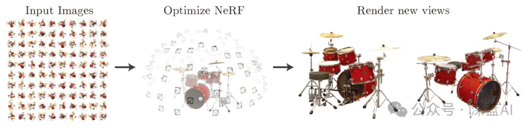
▲图1|NeRF实现流程©️【深蓝AI】
基于前文的原理,本节开始讲述具体的代码实现。首先,导入算法需要的Python库文件。
import osfrom typing import Optional,Tuple,List,Union,Callableimport numpy as npimport torchfrom torch import nnimport matplotlib.pyplot as pltfrom mpl_toolkits.mplot3d import axes3dfrom tqdm import trange# 设置GPU还是CPU设备device = torch.device('cuda' if torch.cuda.is_available() else 'cpu')1 输入
根据相关论文中的介绍可知,NeRF的输入是一个包含空间位置坐标与视图方向的5D坐标。然而,在PyTorch构建NeRF过程中使用的数据集只是一般的3D到2D图像数据集,包含拍摄相机的内参:位姿和焦距。因此在后面的操作中,我们会把输入数据集转为算法模型需要的输入形式。
使用乐高推土机图像作为简单NeRF算法的数据集,在流程中请参考图2。(具体数据链接请见文末)
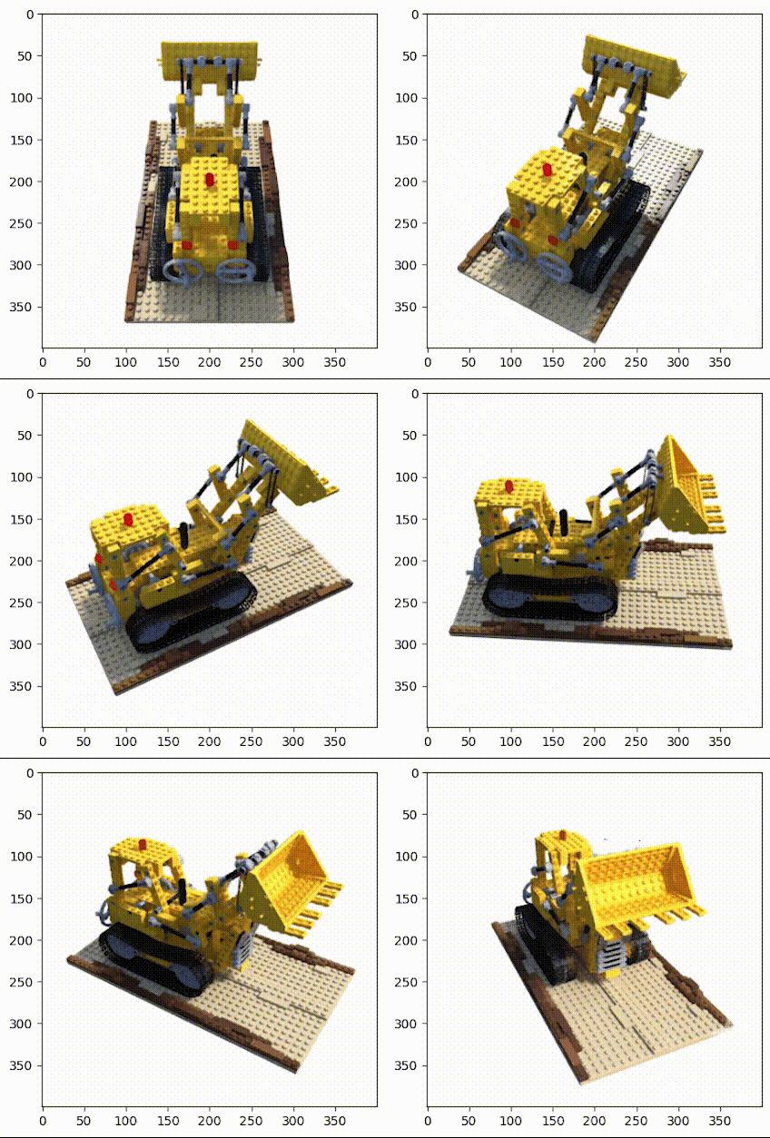
▲图2|乐高推土机数据集©️【深蓝AI】
这项工作中使用的小型乐高数据集由 106 幅乐高推土机的图像组成,并配有位姿数据和常用焦距数值。与其他数据集一样,这里保留前 100 张图像用于训练,并保留一张测试图像用于验证,具体的加载数据操作如下:
data = np.load('tiny_nerf_data.npz') # 加载数据集images = data['images']# 图像数据poses = data['poses']# 位姿数据focal = data['focal']# 焦距数值print(f'Images shape: {images.shape}')print(f'Poses shape: {poses.shape}')print(f'Focal length: {focal}')height, width = images.shape[1:3]near, far = 2., 6.n_training = 100 # 训练数据数量testimg_idx = 101 # 测试数据下标testimg, testpose = images[testimg_idx], poses[testimg_idx]plt.imshow(testimg)print('Pose')print(testpose)2 数据处理
回顾NeRF相关论文,本次代码实现需要的输入是一个单独的5D坐标(空间位置和视图方向)。因此,我们需要针对上面使用的小型乐高数据做一个处理操作。
一般而言,为了收集这些特点输入数据,算法中需要对输入图像进行反渲染操作。具体来讲就是通过每个像素点在三维空间中绘制投影线,并从中提取样本。
要从图像以外的三维空间采样输入数据点,首先就得从乐高照片集中获取每台相机的初始位姿,然后通过一些矢量数学运算,将这些4x4姿态矩阵转换成「表示原点的三维坐标和表示方向的三维矢量」——这两类信息最终会结合起来描述一个矢量,该矢量用以表征拍摄照片时相机的指向。
下列代码则正是通过绘制箭头来描述这一操作,箭头表示每一帧图像的原点和方向:
# 方向数据dirs = np.stack([np.sum([0, 0, -1] * pose[:3, :3], axis=-1) for pose in poses])# 原点数据origins = poses[:, :3, -1]# 绘图的设置ax = plt.figure(figsize=(12, 8)).add_subplot(projectinotallow='3d')_ = ax.quiver(origins[..., 0].flatten(),origins[..., 1].flatten(),origins[..., 2].flatten(),dirs[..., 0].flatten(),dirs[..., 1].flatten(),dirs[..., 2].flatten(), length=0.5, normalize=True)ax.set_xlabel('X')ax.set_ylabel('Y')ax.set_zlabel('z')plt.show()最终绘制出来的箭头结果如下图所示:
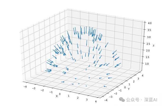
▲图3|采样点相机拍摄指向©️【深蓝AI】
当有了这些相机位姿数据之后,我们就可以沿着图像的每个像素找到投影线,而每条投影线都是由其原点(x,y,z)和方向联合定义。其中每个像素的原点可能相同,但方向一般是不同的。这些方向射线都略微偏离中心,因此不会存在两条平行方向线,如下图所示:
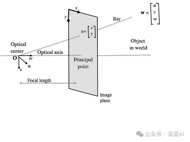
根据图4所述的原理,我们就可以确定每条射线的方向和原点,相关代码如下:
def get_rays(height: int, # 图像高度width: int, # 图像宽带focal_length: float, # 焦距c2w: torch.Tensor) -> Tuple[torch.Tensor, torch.Tensor]:"""通过每个像素和相机原点,找到射线的原点和方向。 """# 应用针孔相机模型收集每个像素的方向i, j = torch.meshgrid(torch.arange(width, dtype=torch.float32).to(c2w),torch.arange(height, dtype=torch.float32).to(c2w),indexing='ij')i, j = i.transpose(-1, -2), j.transpose(-1, -2)# 方向数据directions = torch.stack([(i - width * .5) / focal_length,-(j - height * .5) / focal_length,-torch.ones_like(i) ], dim=-1)# 用相机位姿求出方向rays_d = torch.sum(directions[..., None, :] * c2w[:3, :3], dim=-1)# 默认所有射线原点相同rays_o = c2w[:3, -1].expand(rays_d.shape)return rays_o, rays_d
得到每个像素对应的射线的方向数据和原点数据之后,就能够获得了NeRF算法中需要的五维数据输入,下面将这些数据调整为算法输入的格式:
# 转为PyTorch的tensorimages = torch.from_numpy(data['images'][:n_training]).to(device)poses = torch.from_numpy(data['poses']).to(device)focal = torch.from_numpy(data['focal']).to(device)testimg = torch.from_numpy(data['images'][testimg_idx]).to(device)testpose = torch.from_numpy(data['poses'][testimg_idx]).to(device)# 针对每个图像获取射线height, width = images.shape[1:3]with torch.no_grad():ray_origin, ray_direction = get_rays(height, width, focal, testpose)print('Ray Origin')print(ray_origin.shape)print(ray_origin[height // 2, width // 2, :])print('')print('Ray Direction')print(ray_direction.shape)print(ray_direction[height // 2, width // 2, :])print('')分层采样
当算法输入模块有了NeRF算法需要的输入数据,也就是包含原点和方向向量组合的线条时,就可以在线条上进行采样。这一过程是采用从粗到细的采样策略,即分层采样策略。
具体来说,分层采样就是将光线分成均匀分布的小块,接着在每个小块内随机抽样。其中扰动的设置决定了是均匀取样的,还是直接简单使用分区中心作为采样点。具体操作代码如下所示:
# 采样函数定义def sample_stratified(rays_o: torch.Tensor, # 射线原点rays_d: torch.Tensor, # 射线方向near: float,far: float,n_samples: int, # 采样数量perturb: Optional[bool] = True, # 扰动设置inverse_depth: bool = False# 反向深度) -> Tuple[torch.Tensor, torch.Tensor]:"""从规则的bin中沿着射线进行采样。"""# 沿着射线抓取采样点t_vals = torch.linspace(0., 1., n_samples, device=rays_o.device)if not inverse_depth:# 由远到近线性采样z_vals = near * (1.-t_vals) + far * (t_vals)else:# 在反向深度中线性采样z_vals = 1./(1./near * (1.-t_vals) + 1./far * (t_vals))# 沿着射线从bins中统一采样if perturb:mids = .5 * (z_vals[1:] + z_vals[:-1])upper = torch.concat([mids, z_vals[-1:]], dim=-1)lower = torch.concat([z_vals[:1], mids], dim=-1)t_rand = torch.rand([n_samples], device=z_vals.device)z_vals = lower + (upper - lower) * t_randz_vals = z_vals.expand(list(rays_o.shape[:-1]) + [n_samples])# 应用相应的缩放参数pts = rays_o[..., None, :] + rays_d[..., None, :] * z_vals[..., :, None]return pts, z_vals
接着就到了对这些采样点做可视化分析的步骤。如图5中所述,未受扰动的蓝 色点是bin的“中心“,而红点对应扰动点的采样。请注意,红点与上方的蓝点略有偏移,但所有点都在远近采样设定值之间。具体代码如下:
y_vals = torch.zeros_like(z_vals)# 调用采样策略函数_, z_vals_unperturbed = sample_stratified(rays_o, rays_d, near, far, n_samples,perturb=False, inverse_depth=inverse_depth)# 绘图相关plt.plot(z_vals_unperturbed[0].cpu().numpy(), 1 + y_vals[0].cpu().numpy(), 'b-o')plt.plot(z_vals[0].cpu().numpy(), y_vals[0].cpu().numpy(), 'r-o')plt.ylim([-1, 2])plt.title('Stratified Sampling (blue) with Perturbation (red)')ax = plt.gca()ax.axes.yaxis.set_visible(False)plt.grid(True)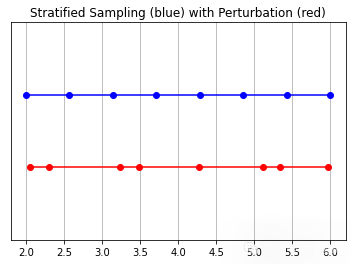
▲图5|采样结果示意图©️【深蓝AI】
3 位置编码
与Transformer一样,NeRF也使用了位置编码器。因此NeRF就需要借助位置编码器将输入映射到更高的频率空间,以弥补神经网络在学习低频函数时的偏差。
这一环节将会为位置编码器建立一个简单的 torch.nn.Module 模块,相同的编码器可同时用于对输入样本和视图方向的编码操作。注意,这些输入被指定了不同的参数。代码如下所示:
# 位置编码类class PositionalEncoder(nn.Module):"""对输入点,做sine或者consine位置编码。"""def __init__(self,d_input: int,n_freqs: int,log_space: bool = False):super().__init__()self.d_input = d_inputself.n_freqs = n_freqsself.log_space = log_spaceself.d_output = d_input * (1 + 2 * self.n_freqs)self.embed_fns = [lambda x: x]# 定义线性或者log尺度的频率if self.log_space:freq_bands = 2.**torch.linspace(0., self.n_freqs - 1, self.n_freqs)else:freq_bands = torch.linspace(2.**0., 2.**(self.n_freqs - 1), self.n_freqs)# 替换sin和cosfor freq in freq_bands:self.embed_fns.append(lambda x, freq=freq: torch.sin(x * freq))self.embed_fns.append(lambda x, freq=freq: torch.cos(x * freq))def forward(self,x) -> torch.Tensor:"""实际使用位置编码的函数。"""return torch.concat([fn(x) for fn in self.embed_fns], dim=-1)
4 NeRF模型
在此,定义一个NeRF 模型——主要由线性层模块列表构成,而列表中进一步包含非线性激活函数和残差连接。该模型有一个可选的视图方向输入,如果在实例化时提供具体的方向信息,那么会改变模型结构。
(本实现基于原始论文NeRF:Representing Scenes as Neural Radiance Fields for View Synthesis 的第3节,并使用相同的默认设置)
具体代码如下所示:
# 定义NeRF模型class NeRF(nn.Module):"""神经辐射场模块。"""def __init__(self,d_input: int = 3,n_layers: int = 8,d_filter: int = 256,skip: Tuple[int] = (4,),d_viewdirs: Optional[int] = None):super().__init__()self.d_input = d_input # 输入self.skip = skip # 残差连接self.act = nn.functional.relu # 激活函数self.d_viewdirs = d_viewdirs # 视图方向# 创建模型的层结构self.layers = nn.ModuleList([nn.Linear(self.d_input, d_filter)] +[nn.Linear(d_filter + self.d_input, d_filter) if i in skip \ else nn.Linear(d_filter, d_filter) for i in range(n_layers - 1)])# Bottleneck 层if self.d_viewdirs is not None:# 如果使用视图方向,分离alpha和RGBself.alpha_out = nn.Linear(d_filter, 1)self.rgb_filters = nn.Linear(d_filter, d_filter)self.branch = nn.Linear(d_filter + self.d_viewdirs, d_filter // 2)self.output = nn.Linear(d_filter // 2, 3)else:# 如果不使用试图方向,则简单输出self.output = nn.Linear(d_filter, 4)def forward(self,x: torch.Tensor,viewdirs: Optional[torch.Tensor] = None) -> torch.Tensor:r"""带有视图方向的前向传播"""# 判断是否设置视图方向if self.d_viewdirs is None and viewdirs is not None:raise ValueError('Cannot input x_direction if d_viewdirs was not given.')# 运行bottleneck层之前的网络层x_input = xfor i, layer in enumerate(self.layers):x = self.act(layer(x))if i in self.skip:x = torch.cat([x, x_input], dim=-1)# 运行 bottleneckif self.d_viewdirs is not None:# Split alpha from network outputalpha = self.alpha_out(x)# 结果传入到rgb过滤器x = self.rgb_filters(x)x = torch.concat([x, viewdirs], dim=-1)x = self.act(self.branch(x))x = self.output(x)# 拼接alpha一起作为输出x = torch.concat([x, alpha], dim=-1)else:# 不拼接,简单输出x = self.output(x)return x5 体积渲染
上面得到NeRF模型的输出结果之后,仍需将NeRF的输出转换成图像。也就是通过渲染模块对每个像素沿光线方向的所有样本进行加权求和,从而得到该像素的估计颜色值,此外每个RGB样本都会根据其Alpha值进行加权。其中Alpha值越高,表明采样区域不透明的可能性越大,因此沿射线方向越远的点越有可能被遮挡,累加乘积可确保更远处的点受到抑制。具体代码如下:
# 体积渲染def cumprod_exclusive(tensor: torch.Tensor) -> torch.Tensor:"""(Courtesy of https://github.com/krrish94/nerf-pytorch)和tf.math.cumprod(..., exclusive=True)功能类似参数:tensor (torch.Tensor): Tensor whose cumprod (cumulative product, see `torch.cumprod`) along dim=-1is to be computed.返回值:cumprod (torch.Tensor): cumprod of Tensor along dim=-1, mimiciking the functionality oftf.math.cumprod(..., exclusive=True) (see `tf.math.cumprod` for details)."""# 首先计算规则的cunprodcumprod = torch.cumprod(tensor, -1)cumprod = torch.roll(cumprod, 1, -1)# 用1替换首个元素cumprod[..., 0] = 1.return cumprod# 输出到图像的函数def raw2outputs(raw: torch.Tensor,z_vals: torch.Tensor,rays_d: torch.Tensor,raw_noise_std: float = 0.0,white_bkgd: bool = False) -> Tuple[torch.Tensor, torch.Tensor, torch.Tensor, torch.Tensor]:"""将NeRF的输出转换为RGB输出。"""# 沿着`z_vals`轴元素之间的差值.dists = z_vals[..., 1:] - z_vals[..., :-1]dists = torch.cat([dists, 1e10 * torch.ones_like(dists[..., :1])], dim=-1)# 将每个距离乘以相应方向射线的法线,转换为现实世界中的距离(考虑非单位方向)。dists = dists * torch.norm(rays_d[..., None, :], dim=-1)# 为模型预测密度添加噪音。可用于在训练过程中对网络进行正则化(防止出现浮点伪影)。noise = 0.if raw_noise_std > 0.:noise = torch.randn(raw[..., 3].shape) * raw_noise_std# Predict density of each sample along each ray. Higher values imply# higher likelihood of being absorbed at this point. [n_rays, n_samples]alpha = 1.0 - torch.exp(-nn.functional.relu(raw[..., 3] + noise) * dists)# 预测每条射线上每个样本的密度。数值越大,表示该点被吸收的可能性越大。[n_ 射线,n_样本]weights = alpha * cumprod_exclusive(1. - alpha + 1e-10)# 计算RGB图的权重。rgb = torch.sigmoid(raw[..., :3])# [n_rays, n_samples, 3]rgb_map = torch.sum(weights[..., None] * rgb, dim=-2)# [n_rays, 3]# 估计预测距离的深度图。depth_map = torch.sum(weights * z_vals, dim=-1)# 稀疏图disp_map = 1. / torch.max(1e-10 * torch.ones_like(depth_map),depth_map / torch.sum(weights, -1))# 沿着每条射线加权。acc_map = torch.sum(weights, dim=-1)# 要合成到白色背景上,请使用累积的 alpha 贴图。if white_bkgd:rgb_map = rgb_map + (1. - acc_map[..., None])return rgb_map, depth_map, acc_map, weights
6 分层体积采样
事实上,三维空间中的遮挡物非常稀疏,因此大多数点对渲染图像的贡献不大。所以,对积分有贡献的区域进行超采样会有更好的效果。这里,笔者对第一组样本应用基于归一化的权重来创建整个光线的概率密度函数,然后对该密度函数应用反变换采样来收集第二组样本。具体代码如下:
# 采样概率密度函数def sample_pdf(bins: torch.Tensor,weights: torch.Tensor,n_samples: int,perturb: bool = False) -> torch.Tensor:"""应用反向转换采样到一组加权点。"""# 正则化权重得到概率密度函数。pdf = (weights + 1e-5) / torch.sum(weights + 1e-5, -1, keepdims=True) # [n_rays, weights.shape[-1]]# 将概率密度函数转为累计分布函数。cdf = torch.cumsum(pdf, dim=-1) # [n_rays, weights.shape[-1]]cdf = torch.concat([torch.zeros_like(cdf[..., :1]), cdf], dim=-1) # [n_rays, weights.shape[-1] + 1]# 从累计分布函数中提取样本位置。perturb == 0 时为线性。if not perturb:u = torch.linspace(0., 1., n_samples, device=cdf.device)u = u.expand(list(cdf.shape[:-1]) + [n_samples]) # [n_rays, n_samples]else:u = torch.rand(list(cdf.shape[:-1]) + [n_samples], device=cdf.device) # [n_rays, n_samples]# 沿累计分布函数找出 u 值所在的索引。u = u.contiguous() # 返回具有相同值的连续张量。inds = torch.searchsorted(cdf, u, right=True) # [n_rays, n_samples]# 夹住超出范围的索引。below = torch.clamp(inds - 1, min=0)above = torch.clamp(inds, max=cdf.shape[-1] - 1)inds_g = torch.stack([below, above], dim=-1) # [n_rays, n_samples, 2]# 从累计分布函数和相应的 bin 中心取样。matched_shape = list(inds_g.shape[:-1]) + [cdf.shape[-1]]cdf_g = torch.gather(cdf.unsqueeze(-2).expand(matched_shape), dim=-1, index=inds_g)bins_g = torch.gather(bins.unsqueeze(-2).expand(matched_shape), dim=-1,index=inds_g)# 将样本转换为射线长度。denom = (cdf_g[..., 1] - cdf_g[..., 0])denom = torch.where(denom < 1e-5, torch.ones_like(denom), denom)t = (u - cdf_g[..., 0]) / denomsamples = bins_g[..., 0] + t * (bins_g[..., 1] - bins_g[..., 0])return samples # [n_rays, n_samples]
7 整体的前向传播流程
此时应将上面所有内容整合在一起,通过模型计算一次前向传递。
由于潜在的内存问题,前向传递以“块“为单位进行计算,然后汇总到一个批次中。梯度传播是在整个批次处理完毕后进行的,因此有“块“和“批次“之分。对于内存紧张环境来说,分块处理尤为重要,因为该环境下提供的资源比原始论文中引用的资源更为有限。具体代码如下所示:
def get_chunks(inputs: torch.Tensor,chunksize: int = 2**15) -> List[torch.Tensor]:"""输入分块。"""return [inputs[i:i + chunksize] for i in range(0, inputs.shape[0], chunksize)]def prepare_chunks(points: torch.Tensor,encoding_function: Callable[[torch.Tensor], torch.Tensor],chunksize: int = 2**15) -> List[torch.Tensor]:"""对点进行编码和分块,为 NeRF 模型做好准备。"""points = points.reshape((-1, 3))points = encoding_function(points)points = get_chunks(points, chunksize=chunksize)return pointsdef prepare_viewdirs_chunks(points: torch.Tensor,rays_d: torch.Tensor,encoding_function: Callable[[torch.Tensor], torch.Tensor],chunksize: int = 2**15) -> List[torch.Tensor]:r"""对视图方向进行编码和分块,为 NeRF 模型做好准备。"""viewdirs = rays_d / torch.norm(rays_d, dim=-1, keepdim=True)viewdirs = viewdirs[:, None, ...].expand(points.shape).reshape((-1, 3))viewdirs = encoding_function(viewdirs)viewdirs = get_chunks(viewdirs, chunksize=chunksize)return viewdirsdef nerf_forward(rays_o: torch.Tensor,rays_d: torch.Tensor,near: float,far: float,encoding_fn: Callable[[torch.Tensor], torch.Tensor],coarse_model: nn.Module,kwargs_sample_stratified: dict = None,n_samples_hierarchical: int = 0,kwargs_sample_hierarchical: dict = None,fine_model = None,viewdirs_encoding_fn: Optional[Callable[[torch.Tensor], torch.Tensor]] = None,chunksize: int = 2**15) -> Tuple[torch.Tensor, torch.Tensor, torch.Tensor, dict]:"""计算一次前向传播"""# 设置参数if kwargs_sample_stratified is None:kwargs_sample_stratified = {}if kwargs_sample_hierarchical is None:kwargs_sample_hierarchical = {}# 沿着每条射线的样本查询点。query_points, z_vals = sample_stratified(rays_o, rays_d, near, far, **kwargs_sample_stratified)# 准备批次。batches = prepare_chunks(query_points, encoding_fn, chunksize=chunksize)if viewdirs_encoding_fn is not None:batches_viewdirs = prepare_viewdirs_chunks(query_points, rays_d, viewdirs_encoding_fn, chunksize=chunksize)else:batches_viewdirs = [None] * len(batches)# 稀疏模型流程。predictions = []for batch, batch_viewdirs in zip(batches, batches_viewdirs):predictions.append(coarse_model(batch, viewdirs=batch_viewdirs))raw = torch.cat(predictions, dim=0)raw = raw.reshape(list(query_points.shape[:2]) + [raw.shape[-1]])# 执行可微分体积渲染,重新合成 RGB 图像。rgb_map, depth_map, acc_map, weights = raw2outputs(raw, z_vals, rays_d)outputs = {'z_vals_stratified': z_vals}if n_samples_hierarchical > 0:# Save previous outputs to return.rgb_map_0, depth_map_0, acc_map_0 = rgb_map, depth_map, acc_map# 对精细查询点进行分层抽样。query_points, z_vals_combined, z_hierarch = sample_hierarchical(rays_o, rays_d, z_vals, weights, n_samples_hierarchical,**kwargs_sample_hierarchical)# 像以前一样准备输入。batches = prepare_chunks(query_points, encoding_fn, chunksize=chunksize)if viewdirs_encoding_fn is not None:batches_viewdirs = prepare_viewdirs_chunks(query_points, rays_d, viewdirs_encoding_fn, chunksize=chunksize)else:batches_viewdirs = [None] * len(batches)# 通过精细模型向前传递新样本。fine_model = fine_model if fine_model is not None else coarse_modelpredictions = []for batch, batch_viewdirs in zip(batches, batches_viewdirs):predictions.append(fine_model(batch, viewdirs=batch_viewdirs))raw = torch.cat(predictions, dim=0)raw = raw.reshape(list(query_points.shape[:2]) + [raw.shape[-1]])# 执行可微分体积渲染,重新合成 RGB 图像。rgb_map, depth_map, acc_map, weights = raw2outputs(raw, z_vals_combined, rays_d)# 存储输出outputs['z_vals_hierarchical'] = z_hierarchoutputs['rgb_map_0'] = rgb_map_0outputs['depth_map_0'] = depth_map_0outputs['acc_map_0'] = acc_map_0# 存储输出outputs['rgb_map'] = rgb_mapoutputs['depth_map'] = depth_mapoutputs['acc_map'] = acc_mapoutputs['weights'] = weightsreturn outputs到这一步骤,就几乎拥有了训练模型所需的一切模块。现在为一个简单的训练过程做一些设置,创建超参数和辅助函数,然后来训练模型。
7.1 超参数
所有用于训练的超参数都在此设置,默认值取自原始论文中数据,除非计算上有限制。在计算受限情况下,本次讨论采用的都是合理的默认值。
# 编码器d_input = 3 # 输入维度n_freqs = 10# 输入到编码函数中的样本点数量log_space = True# 如果设置,频率按对数空间缩放use_viewdirs = True # 如果设置,则使用视图方向作为输入n_freqs_views = 4 # 视图编码功能的数量# 采样策略n_samples = 64 # 每条射线的空间样本数perturb = True # 如果设置,则对采样位置应用噪声inverse_depth = False# 如果设置,则按反深度线性采样点# 模型d_filter = 128# 线性层滤波器的尺寸n_layers = 2# bottleneck层数量skip = [] # 应用输入残差的层级use_fine_model = True # 如果设置,则创建一个精细模型d_filter_fine = 128 # 精细网络线性层滤波器的尺寸n_layers_fine = 6 # 精细网络瓶颈层数# 分层采样n_samples_hierarchical = 64 # 每条射线的样本数perturb_hierarchical = False# 如果设置,则对采样位置应用噪声# 优化器lr = 5e-4# 学习率# 训练n_iters = 10000batch_size = 2**14# 每个梯度步长的射线数量(2 的幂次)one_image_per_step = True # 每个梯度步骤一个图像(禁用批处理)chunksize = 2**14 # 根据需要进行修改,以适应 GPU 内存center_crop = True# 裁剪图像的中心部分(每幅图像裁剪一次)center_crop_iters = 50# 经过这么多epoch后,停止裁剪中心display_rate = 25# 每 X 个epoch显示一次测试输出# 早停warmup_iters = 100# 热身阶段的迭代次数warmup_min_fitness = 10.0 # 在热身_iters 处继续训练的最小 PSNR 值n_restarts = 10 # 训练停滞时重新开始的次数# 捆绑了各种函数的参数,以便一次性传递。kwargs_sample_stratified = {'n_samples': n_samples,'perturb': perturb,'inverse_depth': inverse_depth}kwargs_sample_hierarchical = {'perturb': perturb}7.2 训练类和函数
这一环节会创建一些用于训练的辅助函数。NeRF很容易出现局部最小值,在这种情况下,训练很快就会停滞并产生空白输出。必要时,会利用EarlyStopping重新启动训练。
# 绘制采样函数def plot_samples(z_vals: torch.Tensor,z_hierarch: Optional[torch.Tensor] = None,ax: Optional[np.ndarray] = None):r"""绘制分层样本和(可选)分级样本。"""y_vals = 1 + np.zeros_like(z_vals)if ax is None:ax = plt.subplot()ax.plot(z_vals, y_vals, 'b-o')if z_hierarch is not None:y_hierarch = np.zeros_like(z_hierarch)ax.plot(z_hierarch, y_hierarch, 'r-o')ax.set_ylim([-1, 2])ax.set_title('StratifiedSamples (blue) and Hierarchical Samples (red)')ax.axes.yaxis.set_visible(False)ax.grid(True)return axdef crop_center(img: torch.Tensor,frac: float = 0.5) -> torch.Tensor:r"""从图像中裁剪中心方形。"""h_offset = round(img.shape[0] * (frac / 2))w_offset = round(img.shape[1] * (frac / 2))return img[h_offset:-h_offset, w_offset:-w_offset]class EarlyStopping:r"""基于适配标准的早期停止辅助器"""def __init__(self,patience: int = 30,margin: float = 1e-4):self.best_fitness = 0.0self.best_iter = 0self.margin = marginself.patience = patience or float('inf')# 在epoch停止提高后等待的停止时间def __call__(self,iter: int,fitness: float):r"""检查是否符合停止标准。"""if (fitness - self.best_fitness) > self.margin:self.best_iter = iterself.best_fitness = fitnessdelta = iter - self.best_iterstop = delta >= self.patience# 超过耐性则停止训练return stopdef init_models():r"""为 NeRF 训练初始化模型、编码器和优化器。"""# 编码器encoder = PositionalEncoder(d_input, n_freqs, log_space=log_space)encode = lambda x: encoder(x)# 视图方向编码if use_viewdirs:encoder_viewdirs = PositionalEncoder(d_input, n_freqs_views,log_space=log_space)encode_viewdirs = lambda x: encoder_viewdirs(x)d_viewdirs = encoder_viewdirs.d_outputelse:encode_viewdirs = Noned_viewdirs = None# 模型model = NeRF(encoder.d_output, n_layers=n_layers, d_filter=d_filter, skip=skip,d_viewdirs=d_viewdirs)model.to(device)model_params = list(model.parameters())if use_fine_model:fine_model = NeRF(encoder.d_output, n_layers=n_layers, d_filter=d_filter, skip=skip,d_viewdirs=d_viewdirs)fine_model.to(device)model_params = model_params + list(fine_model.parameters())else:fine_model = None# 优化器optimizer = torch.optim.Adam(model_params, lr=lr)# 早停warmup_stopper = EarlyStopping(patience=50)return model, fine_model, encode, encode_viewdirs, optimizer, warmup_stopper7.3 训练循环
下面就是具体的训练循环过程函数:
def train():r"""启动 NeRF 训练。"""# 对所有图像进行射线洗牌。if not one_image_per_step:height, width = images.shape[1:3]all_rays = torch.stack([torch.stack(get_rays(height, width, focal, p), 0)for p in poses[:n_training]], 0)rays_rgb = torch.cat([all_rays, images[:, None]], 1)rays_rgb = torch.permute(rays_rgb, [0, 2, 3, 1, 4])rays_rgb = rays_rgb.reshape([-1, 3, 3])rays_rgb = rays_rgb.type(torch.float32)rays_rgb = rays_rgb[torch.randperm(rays_rgb.shape[0])]i_batch = 0train_psnrs = []val_psnrs = []iternums = []for i in trange(n_iters):model.train()if one_image_per_step:# 随机选择一张图片作为目标。target_img_idx = np.random.randint(images.shape[0])target_img = images[target_img_idx].to(device)if center_crop and i < center_crop_iters:target_img = crop_center(target_img)height, width = target_img.shape[:2]target_pose = poses[target_img_idx].to(device)rays_o, rays_d = get_rays(height, width, focal, target_pose)rays_o = rays_o.reshape([-1, 3])rays_d = rays_d.reshape([-1, 3])else:# 在所有图像上随机显示。batch = rays_rgb[i_batch:i_batch + batch_size]batch = torch.transpose(batch, 0, 1)rays_o, rays_d, target_img = batchheight, width = target_img.shape[:2]i_batch += batch_size# 一个epoch后洗牌if i_batch >= rays_rgb.shape[0]:rays_rgb = rays_rgb[torch.randperm(rays_rgb.shape[0])]i_batch = 0target_img = target_img.reshape([-1, 3])# 运行 TinyNeRF 的一次迭代,得到渲染后的 RGB 图像。outputs = nerf_forward(rays_o, rays_d, near, far, encode, model, kwargs_sample_stratified=kwargs_sample_stratified, n_samples_hierarchical=n_samples_hierarchical, kwargs_sample_hierarchical=kwargs_sample_hierarchical, fine_model=fine_model, viewdirs_encoding_fn=encode_viewdirs, chunksize=chunksize)# 检查任何数字问题。for k, v in outputs.items():if torch.isnan(v).any():print(f"! [Numerical Alert] {k} contains NaN.")if torch.isinf(v).any():print(f"! [Numerical Alert] {k} contains Inf.")# 反向传播rgb_predicted = outputs['rgb_map']loss = torch.nn.functional.mse_loss(rgb_predicted, target_img)loss.backward()optimizer.step()optimizer.zero_grad()psnr = -10. * torch.log10(loss)train_psnrs.append(psnr.item())# 以给定的显示速率评估测试值。if i % display_rate == 0:model.eval()height, width = testimg.shape[:2]rays_o, rays_d = get_rays(height, width, focal, testpose)rays_o = rays_o.reshape([-1, 3])rays_d = rays_d.reshape([-1, 3])outputs = nerf_forward(rays_o, rays_d, near, far, encode, model, kwargs_sample_stratified=kwargs_sample_stratified, n_samples_hierarchical=n_samples_hierarchical, kwargs_sample_hierarchical=kwargs_sample_hierarchical, fine_model=fine_model, viewdirs_encoding_fn=encode_viewdirs, chunksize=chunksize)rgb_predicted = outputs['rgb_map']loss = torch.nn.functional.mse_loss(rgb_predicted, testimg.reshape(-1, 3))print("Loss:", loss.item())val_psnr = -10. * torch.log10(loss)val_psnrs.append(val_psnr.item())iternums.append(i)# 绘制输出示例fig, ax = plt.subplots(1, 4, figsize=(24,4), gridspec_kw={'width_ratios': [1, 1, 1, 3]})ax[0].imshow(rgb_predicted.reshape([height, width, 3]).detach().cpu().numpy())ax[0].set_title(f'Iteration: {i}')ax[1].imshow(testimg.detach().cpu().numpy())ax[1].set_title(f'Target')ax[2].plot(range(0, i + 1), train_psnrs, 'r')ax[2].plot(iternums, val_psnrs, 'b')ax[2].set_title('PSNR (train=red, val=blue')z_vals_strat = outputs['z_vals_stratified'].view((-1, n_samples))z_sample_strat = z_vals_strat[z_vals_strat.shape[0] // 2].detach().cpu().numpy()if 'z_vals_hierarchical' in outputs:z_vals_hierarch = outputs['z_vals_hierarchical'].view((-1, n_samples_hierarchical))z_sample_hierarch = z_vals_hierarch[z_vals_hierarch.shape[0] // 2].detach().cpu().numpy()else:z_sample_hierarch = None_ = plot_samples(z_sample_strat, z_sample_hierarch, ax=ax[3])ax[3].margins(0)plt.show()# 检查 PSNR 是否存在问题,如果发现问题,则停止运行。if i == warmup_iters - 1:if val_psnr < warmup_min_fitness:print(f'Val PSNR {val_psnr} below warmup_min_fitness {warmup_min_fitness}. Stopping...')return False, train_psnrs, val_psnrselif i < warmup_iters:if warmup_stopper is not None and warmup_stopper(i, psnr):print(f'Train PSNR flatlined at {psnr} for {warmup_stopper.patience} iters. Stopping...')return False, train_psnrs, val_psnrsreturn True, train_psnrs, val_psnrs最终的结果如下图所示:


▲图6|运行结果示意图©️【深蓝AI】

原文链接:https://mp.weixin.qq.com/s/O9ohRJ_TFUoW4cc1GBPuXw













WPS Office是一款面向macOS用户的综合办公套件,将文字处理、电子表格、演示文稿、PDF工具、模板与云协作整合在同一应用中。它兼容常见Microsoft Office格式,支持Intel及Apple芯片Mac,基础功能可免费使用,

Shapr3D是一款面向工业设计、机械工程、建筑概念和三维打印工作流的CAD软件。Mac版采用Parasolid建模内核,支持草图约束、实体建模、工程图、可视化渲染及常见CAD格式交换,并可通过账户在多台设备之间同步项目。

REAPER是Cockos开发的数字音频工作站,提供多轨音频与MIDI录制、剪辑、处理、混音和母带制作工具。Mac版兼容Intel与Apple芯片,支持AU、VST、VST3、CLAP等插件格式,并提供高度可定制的工作流程。

Ableton Live 是面向音乐制作人与现场表演者的数字音频工作站,提供编曲视图、独具特色的现场视图、音频录制、MIDI创作、实时变速、乐器及效果器。Mac版原生支持Apple芯片,并可连接音频接口、MIDI控制器和第三方插件。

Adobe After Effects 是面向动态图形、影视特效与视频合成的专业创作软件。它提供关键帧动画、遮罩抠像、运动跟踪、三维空间、文字动画和表达式等工具,并可与 Premiere Pro、Photoshop、Illustrator

Adobe Audition 是面向播客、影视后期、音乐制作及内容创作者的专业音频工作站,提供波形精修、多轨录制与混音、频谱编辑、降噪修复、响度匹配和效果处理工具,并可与 Adobe Premiere 协同完成视频声音制作。

Adobe Bridge 是面向摄影师、设计师及内容团队的免费数字资产管理工具,可集中预览照片、视频和 Adobe 项目文件,并利用评级、标签、关键词、元数据、筛选与收藏集完成分类检索。它还支持批量重命名、格式导出、相机导入及 Camera

Adobe Illustrator 是 Adobe 推出的专业矢量图形设计软件,适合在 Mac 上制作标志、图标、插画、包装、信息图及印刷版面。它以路径和锚点构建可无损缩放的图形,并提供钢笔、形状、文字、图像描摹、渐变、画板及生成式功能。

Adobe InDesign 是面向印刷品与数字出版物的专业版面设计软件,可在 Mac 上制作书籍、杂志、宣传册、海报、报告及交互式文档。它提供精细的文字样式、网格、母版、长文档管理和印前输出能力。

Adobe Lightroom Classic 是面向桌面摄影工作流的照片管理与后期处理软件,可将原始照片保存在本地硬盘,通过目录、关键词、评分和收藏夹高效整理图库,并提供 RAW 冲印、蒙版、镜头校正、批量同步及多格式导出等功能。

Adobe Media Encoder 是 Adobe 推出的专业音视频编码与转码工具,可通过队列、预设和监视文件夹批量完成格式转换、代理文件创建及多平台成片输出,并与 Premiere Pro、After Effects 等软件紧密协作。

Adobe Photoshop 是面向摄影师、设计师和内容创作者的专业图像处理软件,提供图层、蒙版、选区、修复、调色、文字排版、智能对象及生成式编辑等能力。Mac 版支持 Intel 与 Apple Silicon 处理器。

Adobe Photoshop 是面向摄影师、设计师和内容创作者的专业图像处理工具,可在 Windows 上完成照片修饰、选区抠图、图层合成、文字排版、绘画及生成式编辑。软件采用订阅授权,由 Creative Cloud 管理安装、更新与许

Adobe InDesign 是面向印刷与数字出版的专业页面排版工具,可制作书籍、杂志、宣传册、海报、交互式 PDF 和电子书。它提供精细的文字样式、多页面管理、印前检查及多格式输出能力,并能与 Photoshop、Illustrator

Adobe Illustrator 是用于绘制矢量图形、插画、图标、徽标和版式的专业设计工具。它以路径和锚点为核心,作品放大后仍能保持清晰,并提供画板、文字、渐变、图像描摹及精确变换等功能,适合品牌视觉、印刷物料、数字界面和商业插画创作。

Adobe Bridge 是 Adobe 推出的创意资产管理工具,可集中预览、分类和查找照片、视频、PDF及多种设计文件,并支持元数据、关键词、评级、批量重命名和格式导出。它可与 Photoshop、Illustrator 等应用衔接,

Affinity Photo 是一款面向摄影师、修图师和视觉设计人员的桌面图像编辑工具,提供 RAW 显影、多图层合成、蒙版、实时滤镜、批处理和色彩管理等功能。原独立产品已停止销售,其照片编辑能力已延续至免费的新 Affinity 应用;

Adobe Lightroom Classic 是面向 Windows 桌面摄影工作流的照片管理与无损编辑工具,可通过目录集中整理大型图库,并完成 RAW 显影、局部蒙版、批量调整、打印和多格式导出。它强调本地文件管理与精细控制,

Figma 是面向产品设计与开发团队的云端协作平台,可在 Windows 桌面客户端中完成界面绘制、组件管理、交互原型、评论评审和开发交付。文件保存在云端,多名成员能够同步编辑并共享设计系统;官方同时提供免费 Starter 方案及按席位计

Affinity Designer 是面向矢量图形、数字插画和界面设计的专业创作工具,可在矢量、像素与导出工作区之间快速切换。它提供曲线编辑、形状构建、画板、排版、图层和专业色彩管理,并支持常见设计文件的导入及多种印刷、网页格式输出。

Capture One Pro 是面向摄影师和影像团队的专业桌面照片处理工具,提供相机定制色彩配置、RAW转换、图层与蒙版、联机拍摄、目录及会话管理等功能。它适合棚拍、人像、商业产品、婚礼和风光摄影,

Adobe Acrobat Pro 是面向专业 PDF 工作的综合解决方案,可在 Windows 中创建、编辑、转换、比较、整理和保护文档,并支持表单、电子签名、扫描件文字识别及敏感信息永久遮盖。订阅还包含网页、移动服务和云端协作能力,

Adobe After Effects 是面向动态图形、动画与影视视觉特效制作的专业工具,可完成关键帧动画、图层合成、遮罩跟踪、抠像、文字动画和二维三维元素整合。Windows 版通过 Adobe Creative Cloud 安装及更新,

DaVinci Resolve是Blackmagic Design推出的一体化影视后期工具,将素材管理、非线性剪辑、专业调色、Fusion视觉特效、Fairlight音频处理和成片交付整合在统一工程中。免费版已覆盖多数个人创作需求,